7.22. Prim’s Spanning Tree Algorithm
For our last graph algorithm let’s consider a problem that online game designers and Internet radio providers face. The problem is that they want to efficiently transfer a piece of information to anyone and everyone who may be listening. This is important in gaming so that all the players know the very latest position of every other player. This is important for Internet radio so that all the listeners that are tuned in are getting all the data they need to reconstruct the song they are listening to. Figure 9 illustrates the broadcast problem.
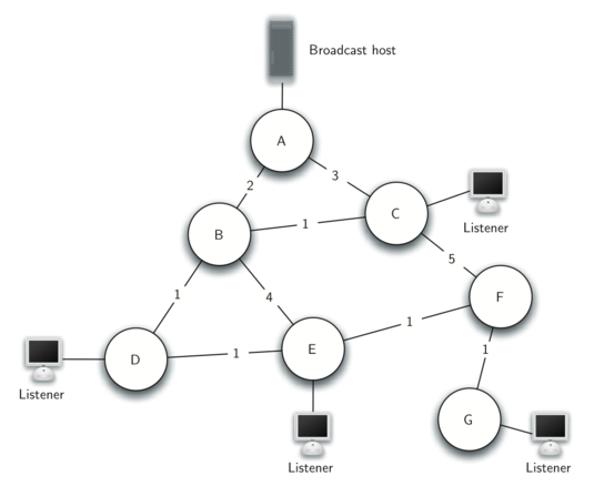
Figure 9: The Broadcast Problem
There are some brute force solutions to this problem, so let’s look at them first to help understand the broadcast problem better. This will also help you appreciate the solution that we will propose when we are done. To begin, the broadcast host has some information that the listeners all need to receive. The simplest solution is for the broadcasting host to keep a list of all of the listeners and send individual messages to each. In Figure 9 we show a small network with a broadcaster and some listeners. Using this first approach, four copies of every message would be sent. Assuming that the least cost path is used, let’s see how many times each router would handle the same message.
All messages from the broadcaster go through router A, so A sees all four copies of every message. Router C sees only one copy of each message for its listener. However, routers B and D would see three copies of every message since routers B and D are on the cheapest path for listeners 1, 2, and 3. When you consider that the broadcast host must send hundreds of messages each second for a radio broadcast, that is a lot of extra traffic.
A brute force solution is for the broadcast host to send a single copy
of the broadcast message and let the routers sort things out. In this
case, the easiest solution is a strategy called uncontrolled
flooding. The flooding strategy works as follows. Each message starts
with a time to live (ttl) value set to some number greater than or
equal to the number of edges between the broadcast host and its most
distant listener. Each router gets a copy of the message and passes the
message on to all of its neighboring routers. When the message is
passed on the ttl is decreased. Each router continues to send copies
of the message to all its neighbors until the ttl value reaches 0.
It is easy to convince yourself that uncontrolled flooding generates
many more unnecessary messages than our first strategy.
The solution to this problem lies in the construction of a minimum weight spanning tree. Formally we define the minimum spanning tree \(T\) for a graph \(G = (V,E)\) as follows. \(T\) is an acyclic subset of \(E\) that connects all the vertices in \(V\). The sum of the weights of the edges in T is minimized.
Figure 10 shows a simplified version of the broadcast graph and highlights the edges that form a minimum spanning tree for the graph. Now to solve our broadcast problem, the broadcast host simply sends a single copy of the broadcast message into the network. Each router forwards the message to any neighbor that is part of the spanning tree, excluding the neighbor that just sent it the message. In this example A forwards the message to B. B forwards the message to D and C. D forwards the message to E, which forwards it to F, which forwards it to G. No router sees more than one copy of any message, and all the listeners that are interested see a copy of the message.
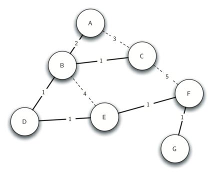
Figure 10: Minimum Spanning Tree for the Broadcast Graph
The algorithm we will use to solve this problem is called Prim’s algorithm. Prim’s algorithm belongs to a family of algorithms called the “greedy algorithms” because at each step we will choose the cheapest next step. In this case the cheapest next step is to follow the edge with the lowest weight. Our last step is to develop Prim’s algorithm.
The basic idea in constructing a spanning tree is as follows:
While T is not yet a spanning tree
   Find an edge that is safe to add to the tree
   Add the new edge to T
The trick is in the step that directs us to “find an edge that is safe.” We define a safe edge as any edge that connects a vertex that is in the spanning tree to a vertex that is not in the spanning tree. This ensures that the tree will always remain a tree and therefore have no cycles.
The Python code to implement Prim’s algorithm is shown in Listing 2. Prim’s algorithm is similar to Dijkstra’s algorithm in that they both use a priority queue to select the next vertex to add to the growing graph.
Listing 2
from pythonds.graphs import PriorityQueue, Graph, Vertex

def prim(G,start):
    pq = PriorityQueue()
    for v in G:
        v.setDistance(sys.maxsize)
        v.setPred(None)
    start.setDistance(0)
    pq.buildHeap([(v.getDistance(),v) for v in G])
    while not pq.isEmpty():
        currentVert = pq.delMin()
        for nextVert in currentVert.getConnections():
          newCost = currentVert.getWeight(nextVert)
          if nextVert in pq and newCost<nextVert.getDistance():
              nextVert.setPred(currentVert)
              nextVert.setDistance(newCost)
              pq.decreaseKey(nextVert,newCost)
The following sequence of figures (Figure 11 through Figure 17) shows the algorithm in operation on our sample tree. We begin with the starting vertex as A. The distances to all the other vertices are initialized to infinity. Looking at the neighbors of A we can update distances to two of the additional vertices B and C because the distances to B and C through A are less than infinite. This moves B and C to the front of the priority queue. Update the predecessor links for B and C by setting them to point to A. It is important to note that we have not formally added B or C to the spanning tree yet. A node is not considered to be part of the spanning tree until it is removed from the priority queue.
Since B has the smallest distance we look at B next. Examining B’s neighbors we see that D and E can be updated. Both D and E get new distance values and their predecessor links are updated. Moving on to the next node in the priority queue we find C. The only node C is adjacent to that is still in the priority queue is F, thus we can update the distance to F and adjust F’s position in the priority queue.
Now we examine the vertices adjacent to node D. We find that we can update E and reduce the distance to E from 6 to 4. When we do this we change the predecessor link on E to point back to D, thus preparing it to be grafted into the spanning tree but in a different location. The rest of the algorithm proceeds as you would expect, adding each new node to the tree.
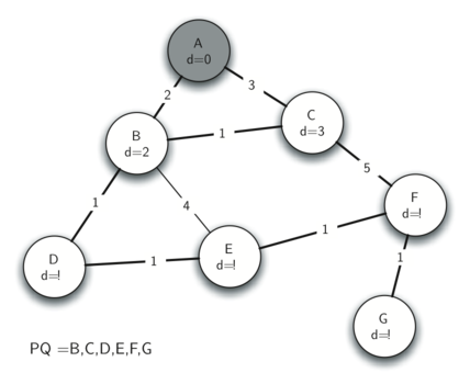
Figure 11: Tracing Prim’s Algorithm
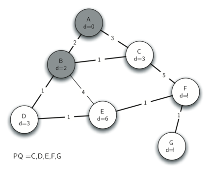
Figure 12: Tracing Prim’s Algorithm
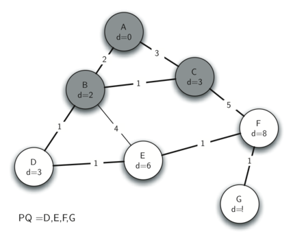
Figure 13: Tracing Prim’s Algorithm
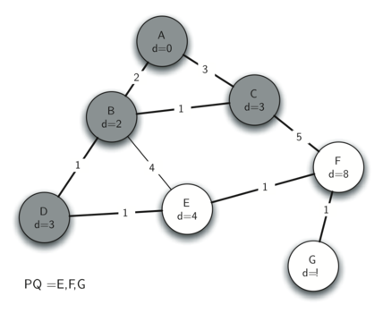
Figure 14: Tracing Prim’s Algorithm
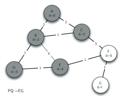
Figure 15: Tracing Prim’s Algorithm
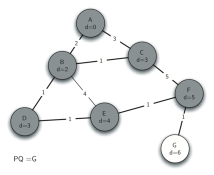
Figure 16: Tracing Prim’s Algorithm
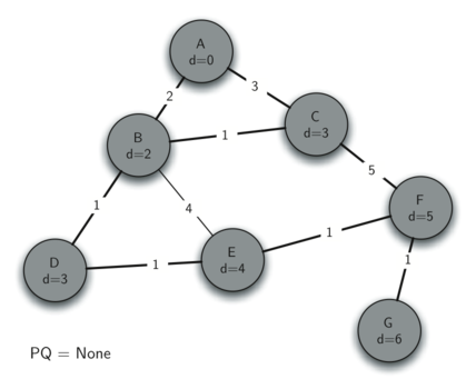
Figure 17: Tracing Prim’s Algorithm